Clustering: k-means and evaluation
How k-means groups unlabelled data, why seeding changes the answer, how to choose k with the elbow and silhouette, and where it fails, with real numbers from a NumPy implementation.
K-means clustering splits unlabelled data into k groups by repeatedly assigning each point to its nearest centroid and moving each centroid to the mean of its points. Interviewers expect the convergence detail: inertia never rises, so the loop always stops, but only at a local minimum that depends on the starting centroids, which is why k-means++ seeding and restarts matter.
K-means splits unlabelled data into k groups by repeatedly assigning points to the nearest centroid and moving each centroid to its group's mean. It always stops, but only at a local minimum, so seeding, the choice of k and feature scaling decide whether the result means anything.
- K-means minimises inertia, the sum of squared distances from each point to its own centroid, and neither step of Lloyd's algorithm can increase it.
- On 600 points in four blobs over 200 seeds, 52% of random-init k-means runs ended within 1% of the best inertia of 913.2, against 92% with k-means++ seeding.
- On the four-blob data, k-means inertia fell from 5018 at k=3 to 913 at k=4 and then barely moved, and the silhouette score peaked at k=4 with 0.830.
- The silhouette of a sample is (b - a) / max(a, b), where a is its mean distance within its own cluster and b its mean distance to the nearest other cluster.
- On two interleaved half-moons, k-means reached an adjusted Rand index of only 0.245, while DBSCAN with eps=0.2 recovered both moons with an index of 1.0.
- In recent scikit-learn, n_init='auto' runs k-means 10 times for init='random' but only once for the default init='k-means++'.
01Grouping points when nobody gave you labels
Say you have 600 customers described by two numbers each, such as orders per month and average basket size, and nobody has told you which customers are alike. Clustering is the task of splitting them into groups so that points inside a group are close to each other and points in different groups are far apart. There is no label column, so you cannot compute accuracy. That single fact shapes the whole topic: every question below (how many groups, is this grouping any good, did the algorithm fool me) has to be answered without a ground truth. If you have worked through the train-test split and cross-validation topic, notice what is missing: there is no held-out label to score against, so those evaluation habits do not carry over directly, and this article swaps in other checks.
K-means is the simplest and most common answer. You pick a number k up front. The algorithm returns k centroids (points that stand for the centre of each group) and assigns every sample to its nearest centroid. It is a flat, hard clustering: no hierarchy, and every point belongs to exactly one group.
To make the rest concrete, all the numbers in this article come from one synthetic dataset, built with make_blobs(n_samples=600, centers=4, cluster_std=0.9, random_state=7) from scikit-learn: four blobs in a plane. Because we generated it, we know the right answer is k=4, which lets us test whether our evaluation tools find it. Real data never tells you that. Exact figures depend on library versions and seeds; these were produced with Python 3, NumPy 2.5.3 and scikit-learn 1.9.1.
02Lloyd's algorithm and the quantity it minimises
K-means chooses centroids that minimise inertia, the within-cluster sum of squared distances: for every point, take the squared distance to its own centroid and add them all up. The scikit-learn docs describe it as a measure of how internally coherent the clusters are. The standard procedure for minimising it is Lloyd's algorithm:
- Choose k starting centroids (the simplest way is k random samples).
- Assignment step: give every point to its nearest centroid.
- Update step: move each centroid to the mean of the points assigned to it.
- Repeat steps 2 and 3 until the centroids stop moving.
Why does it stop? The assignment step picks, for fixed centroids, the closest centroid for each point, so inertia cannot rise. The update step uses the fact that, for a fixed group of points, the mean is the single location with the smallest total squared distance, so inertia cannot rise there either. The objective only goes down or stays flat, and there are finitely many ways to partition the points, so the loop must end. The Stanford IR book makes the same argument for its RSS objective.
Here is the whole algorithm in NumPy, short enough to read in one sitting. An empty cluster simply keeps its old centroid.
import numpy as np
from sklearn.datasets import make_blobs
from sklearn.cluster import KMeans
from sklearn.metrics import silhouette_score

X, y = make_blobs(n_samples=600, centers=4, cluster_std=0.9, random_state=7)

def sqdist(X, C):
    return ((X[:, None, :] - C[None]) ** 2).sum(axis=2)

def lloyd(X, k, seed):
    rng = np.random.default_rng(seed)
    C = X[rng.choice(len(X), k, replace=False)].copy()
    for _ in range(300):
        lab = sqdist(X, C).argmin(axis=1)
        new = np.array([X[lab == j].mean(axis=0) if (lab == j).any() else C[j]
                        for j in range(k)])
        if ((new - C) ** 2).sum() < 1e-6:
            break
        C = new
    d = sqdist(X, C)
    lab = d.argmin(axis=1)
    return lab, d[np.arange(len(X)), lab].sum()
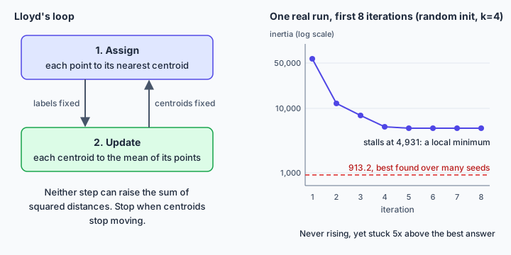
I also logged inertia after every assignment step for one run with random seeding (seed 1, k=4). It went 58960.2, 11803.0, 7715.4, 5133.4, 4933.2, 4931.8, 4931.4, 4931.2 and kept creeping down to 4931.0 over 11 iterations. Never up, as promised. The diagram shows that run next to the loop. Notice the final value, though. The best inertia for this data is 913.2, and this run stopped at 4,931, more than five times higher, with no warning. Stopping only means that no single assign or update step can lower inertia from where the centroids are; it says nothing about whether a different start would reach a far lower value.
03Local minima: why the seed matters
The scikit-learn documentation says it plainly: given enough time k-means will always converge, but possibly to a local minimum, and this depends heavily on initialisation. The picture in our dataset is easy to imagine. If two of the four starting centroids both land inside the same blob, they split it between them, and one other centroid ends up trying to cover two blobs. Neither step of Lloyd's loop can climb out of that arrangement, because each step only ever improves things locally.
The fix has two layers. First, seed more cleverly. The k-means++ method, from the paper by Arthur and Vassilvitskii, picks the first centroid uniformly at random, then picks each following centroid from the data with probability proportional to its squared distance to the nearest centroid already chosen. Far-away points are more likely to be picked, so seeds spread out. The authors prove this is O(log k)-competitive with the optimal clustering and report that it often improves both speed and accuracy dramatically. Second, restart: run the whole thing several times and keep the run with the lowest inertia. In scikit-learn that is n_init.
How much does it help? I ran my own implementations of both seeding methods on the four-blob data, one run per seed, for 200 seeds, and compared inertia against the best value found (913.2). A run counts as good when its final inertia is within 1% of 913.2, that is, at most 922.3. These are my measurements, not library claims, and the code below (which reuses sqdist and X from the previous section) reproduces them exactly.
| Seeding | Within 1% of 913.2 | Worst run | Mean iterations |
|---|---|---|---|
| random samples | 52% of runs | 13983.6 | 6.9 |
| k-means++ | 92% of runs | 4936.7 | 2.8 |
def kpp_seeds(X, k, rng):            # k-means++ seeding (D^2 weighting)
    C = [X[rng.integers(len(X))]]
    for _ in range(k - 1):
        d2 = sqdist(X, np.array(C)).min(axis=1)
        C.append(X[rng.choice(len(X), p=d2 / d2.sum())])
    return np.array(C)

def run(X, k, seed, init):           # one Lloyd run -> (inertia, iterations)
    rng = np.random.default_rng(seed)
    C = X[rng.choice(len(X), k, replace=False)] if init == "random" else kpp_seeds(X, k, rng)
    for it in range(1, 301):
        lab = sqdist(X, C).argmin(axis=1)
        new = np.array([X[lab == j].mean(axis=0) if (lab == j).any() else C[j] for j in range(k)])
        if ((new - C) ** 2).sum() < 1e-6:
            break
        C = new
    return sqdist(X, C).min(axis=1).sum(), it

for init in ["random", "k-means++"]:
    r = np.array([run(X, 4, s, init) for s in range(200)])
    print(init, f"{(r[:, 0] <= 913.2 * 1.01).mean():.0%}", round(r[:, 0].max(), 1), round(r[:, 1].mean(), 1))
Output: random 52% 13983.6 6.9 and k-means++ 92% 4936.7 2.8.
Half of all single random runs were fine, a sizeable minority were awful, and k-means++ fixed most but not all of it. On a harder dataset (1500 points, 10 overlapping blobs, k=10, 100 seeds) neither method was reliable alone: only about 9% of random runs and 10% of k-means++ runs landed within 1% of the best inertia I found (1286.3). The k-means++ median was much lower than the random one (1550.2 against 2110.0), but the spread stayed wide. So use both layers. One detail that surprises people: in recent scikit-learn, n_init='auto' means 10 runs for init='random' but only 1 run for the default init='k-means++' (the default changed in version 1.4). Many older tutorials assume ten runs. If your clusters matter, set n_init=10 yourself.
04Choosing k: elbow versus silhouette
You might hope to try several k and keep the one with the lowest inertia. That fails immediately: more centroids always fit the points at least as well, and with k equal to the number of samples inertia is exactly zero. Inertia is also not normalised, so comparing it between different k tells you nothing by itself. It is only meaningful at a fixed k.
The elbow method plots inertia against k and looks for the point where the curve stops dropping steeply. The silhouette gives a second opinion. For one sample, let a be its mean distance to the other points in its own cluster and b its mean distance to the points of the nearest other cluster. Its silhouette is (b - a) / max(a, b). A value near +1 means the sample sits well inside its cluster, near 0 means it is on a border, and negative values suggest it may be in the wrong cluster. Averaged over all samples, the score ranges from -1 to 1, and it is only defined for 2 <= k <= n_samples - 1. Rousseeuw's paper introduced it as a way to judge cluster validity and possibly choose the number of clusters.
Running the snippet above for each k, taking the best of 10 random seedings, and comparing with scikit-learn's KMeans(k, n_init=10, random_state=0):
for k in range(2, 9):
    best = min((lloyd(X, k, s) for s in range(10)), key=lambda r: r[1])
    sk = KMeans(k, n_init=10, random_state=0).fit(X)
    print(k, round(best[1], 1), round(sk.inertia_, 1), round(silhouette_score(X, best[0]), 3))
| k | my inertia | sklearn inertia | silhouette |
|---|---|---|---|
| 2 | 18162.5 | 18162.5 | 0.594 |
| 3 | 5018.2 | 5018.2 | 0.773 |
| 4 | 913.2 | 913.2 | 0.830 |
| 5 | 826.0 | 826.1 | 0.696 |
| 6 | 741.7 | 745.7 | 0.583 |
| 7 | 662.6 | 663.4 | 0.443 |
| 8 | 611.7 | 590.0 | 0.452 |
The elbow is unmistakable: inertia collapses from 5018 to 913 going from three to four clusters and then barely moves. The silhouette peaks at k=4 with 0.830. My version agrees with scikit-learn up to k=4 and drifts afterwards (at k=8 it is 611.7 against 590.0) because best-of-10 random seeding sometimes keeps a worse local minimum, which is the previous section again.
This dataset is the friendly case. Real data rarely gives such a clean bend, and the average silhouette can mislead too: the scikit-learn silhouette example gives k=2 the highest average (0.7050) even though its per-cluster plots favour k=4. Treat both tools as evidence, and let what the clusters mean for your problem break ties.
05When k-means breaks
The inertia objective builds in an assumption: clusters are convex and roughly isotropic, meaning round blobs. The scikit-learn docs warn that it responds poorly to elongated clusters and manifolds with irregular shapes. Three experiments show what that looks like.
Shape. make_moons(500, noise=0.07, random_state=0) gives two interleaved half-circles. With KMeans(2, n_init=10, random_state=0) the adjusted Rand index against the true labels was 0.245 (1.0 is a perfect match, around 0 is chance). K-means draws a straight boundary through the middle of both crescents. The unpleasant part is what silhouette says. The k-means split scored 0.487, while the correct labelling scored only 0.328, because points at opposite ends of one crescent are far from each other. Silhouette shares k-means's preference for compact shapes, so it endorsed the wrong answer. DBSCAN(eps=0.2), which grows clusters from dense neighbourhoods, recovered both moons with an index of 1.0 on this data.
from sklearn.datasets import make_moons
from sklearn.cluster import DBSCAN
from sklearn.metrics import adjusted_rand_score as ari

Xm, ym = make_moons(500, noise=0.07, random_state=0)
km = KMeans(2, n_init=10, random_state=0).fit_predict(Xm)
print(round(ari(ym, km), 3), round(silhouette_score(Xm, km), 3), round(silhouette_score(Xm, ym), 3))
print(round(ari(ym, DBSCAN(eps=0.2).fit_predict(Xm)), 3))
Output: 0.245 0.487 0.328, then 1.0.
Scale. I built two groups of 200 points that differ clearly in the first feature (means 0 and 5, standard deviation 1) and added a second feature that is pure noise with standard deviation 1000. Euclidean distance is dominated by the big feature. K-means on the raw data scored an adjusted Rand index of -0.002, which is chance (about 0). After StandardScaler, it scored 0.97. With generator seeds 0 to 4 the raw score stayed between -0.002 and 0.008 and the scaled one between 0.951 and 0.99. Standardise features before k-means unless their units are meant to be comparable.
from sklearn.preprocessing import StandardScaler

rng = np.random.default_rng(0)
g = np.repeat([0, 1], 200)                         # true group of each point
Xs = np.column_stack([rng.normal(5 * g, 1),        # signal: means 0 and 5, std 1
                      rng.normal(0, 1000, 400)])   # noise: std 1000
fit = lambda Z: KMeans(2, n_init=10, random_state=0).fit_predict(Z)
print(round(ari(g, fit(Xs)), 3), round(ari(g, fit(StandardScaler().fit_transform(Xs))), 3))
Output: -0.002 0.97.
Outliers and categories. Centroids are means, and a mean gets dragged toward extreme points. The Stanford IR book notes that an outlier chosen as a seed often ends up as a singleton cluster. I did not run an experiment on this, so treat it as a known weakness rather than a measured one. Removing outliers first is one option, and other methods such as k-medoids exist; I have not tested them here. For categorical features, the mean of a set of category values is not defined, so k-means does not apply as it stands. Other algorithms exist for that case, which this article does not cover.
06Cost and practical notes
The IR book puts one iteration at roughly Theta(KNM) work, where K is the number of clusters, N the number of points and M the number of dimensions: every point is compared against every centroid across every coordinate. With I iterations the total is Theta(IKNM). That is linear in each factor, which keeps k-means cheap next to methods that need all pairwise distances. My NumPy version builds an N by K by M temporary array in sqdist, so memory can be the first limit on a big dataset.
A worked example makes the formula concrete. On the four-blob data N=600, K=4 and M=2, so one assignment step computes 600 x 4 x 2 = 4,800 squared coordinate differences. The random-init runs in the seeding table averaged 6.9 iterations, about 33,000 of those operations per run; the k-means++ runs averaged 2.8, about 13,400, plus the seeding passes. The temporary inside sqdist has shape (600, 4, 2): 4,800 float64 values, or 38,400 bytes (checked with .nbytes). Trivial here. Now take N=1,000,000, K=100 and M=50. The arithmetic is still linear, but the same line would want 5 billion values, about 40 GB, for a single iteration. Processing the points in chunks of rows caps that memory at the cost of a loop; I have not checked how scikit-learn organises this internally. Timing follows the linear rule too: on my machine one sqdist call with K=4 and M=2 took about 0.09 ms at N=600, 0.83 ms at N=6,000 and 8.7 ms at N=60,000, so ten times the points cost roughly ten times the time. Those timings are machine-specific; the ratio is the point.
Dimensionality is the usual practical trouble. In very high dimensions Euclidean distances between points become similar and uninformative, and the scikit-learn docs suggest running PCA first, which also speeds the algorithm up.
Empty clusters can happen when a centroid ends up with no points. The IR book counts it as a suboptimal outcome. My code leaves that centroid where it was; other strategies exist, and I have not verified which one scikit-learn uses, so I make no claim about it.
A short checklist before you trust a clustering: scale the features, remove or flag outliers, seed with k-means++ and use several restarts, compare inertia and silhouette across a range of k, then look at the clusters themselves (sizes, centres, a few example rows) and ask whether they make sense for the business or research question. Inertia is also useful in a second way: fixed k, restarts, lowest value wins. That is the only comparison it supports.
07Common interview questions
Q: Explain k-means and say whether it converges.
A: Pick k centroids, assign each point to its nearest one, move each centroid to the mean of its points, and repeat. The sum of squared distances (inertia) cannot increase in either step, so the loop terminates, but only at a local minimum that depends on the starting centroids.
Q: Why can two runs give different clusters, and how do you handle it?
A: The objective has many local minima and the start is random. Use k-means++ seeding, which favours well-spread starting points, and run several restarts keeping the lowest inertia. For example, on 600 points in four well-separated blobs, about half of single random-init runs end within 1% of the best inertia, against roughly nine in ten with k-means++. So even with k-means++, a few restarts are cheap insurance.
Q: Why can't you choose k by taking the lowest inertia?
A: Inertia falls as k rises and reaches zero when every point is its own cluster. Look for the elbow where the drop flattens, and confirm with the average silhouette score. On data with four clear blobs, for instance, inertia drops steeply from three clusters to four and then flattens, and the silhouette peaks at four.
Q: How do you read a silhouette score, and when is it misleading?
A: It is (b - a) / max(a, b) per sample, where a is the mean distance within the cluster and b the mean distance to the nearest other cluster. Near 1 is well clustered, near 0 is overlapping, negative suggests misassignment. It prefers compact convex clusters. On two interleaved half-moons, for example, the correct labelling can score a lower average silhouette (around 0.33) than a wrong straight-line k-means split (around 0.49). The average can also hide uneven cluster sizes.
Q: When does k-means fail, and what do you use instead?
A: It struggles with non-convex shapes, clusters of very different density, outliers and features on different scales. For curved shapes like two interleaved moons, density-based methods such as DBSCAN work better: on a clean example DBSCAN can recover both groups exactly, while k-means agrees with the true labels only weakly (an adjusted Rand index around 0.25).
Q: What preprocessing do you apply before k-means?
A: Standardise numeric features, because Euclidean distance lets a large-scale feature dominate (for example, if one useful feature has a standard deviation of 1 and a noise feature has 1000, k-means on raw data matches the true groups no better than chance, and after standardising it gets them almost all right), and consider PCA for many dimensions.