Feature Engineering and Encoding

A logistic regression multiplies each input by a weight. A k-nearest-neighbours model measures distances. A gradient-boosted tree compares values with thresholds. None of them can use the string "Pune" or a timestamp directly, so every column must become numbers first. That is feature engineering; encoding is the part that handles categories.

The choice is not cosmetic. A bad encoding rarely raises an error; it produces a quietly worse model, or one that shines in the notebook and fails on new data.

Every experiment below uses one synthetic dataset of 6,000 food-delivery orders with a fixed seed. Lateness depends on the restaurant (400 of them, each with its own late rate), distance, a late-evening rush, and whether the restaurant is new. Two columns are traps: customer_id is pure noise and order_value has no effect. Known rules let us see when an encoding helps and when it fools us. The snippets run in order in one Python session (scikit-learn 1.9.1, pandas 3.1.0, NumPy 2.5.4).

35.1% of orders are late, and 2,273 customer IDs share the 6,000 orders, about 2.6 orders each.

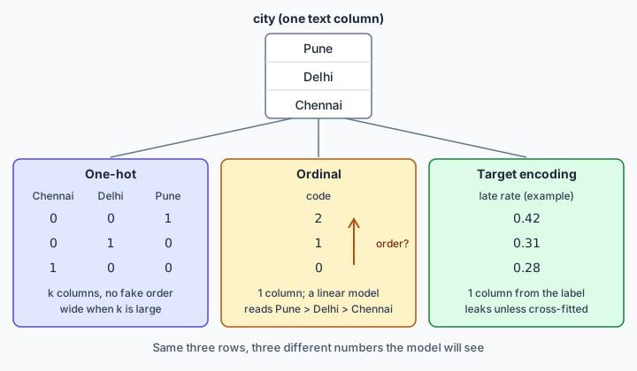
One-hot encoding gives each category its own 0/1 column. Ordinal encoding replaces each category with one integer, in sorted order. That suits a truly ordered column such as small, medium, large. For restaurant names it claims r399 is "more" than r001, which means nothing.

Here a logistic regression sees only the restaurant column, encoded each way, scored by test AUC on a 70/30 split (0.5 is a coin flip):

With one-hot columns the model learns a weight per restaurant and reaches 0.63. Given ordinal codes, it can only fit one slope along an arbitrary line from r000 to r399, so the signal vanishes and the score lands at chance (0.476). Target encoding, covered next, matches one-hot with a single column.

Trees do better with ordinal codes (0.599) because they can cut the integer line into ranges, but they still trail one-hot. With about 10 training orders per restaurant, isolating one bad restaurant needs two cuts between unrelated neighbours, and there is rarely enough data to justify them.

Two settings matter in production. handle_unknown decides what happens to a category never seen in training: raise an error, emit an all-zero row (ignore), or map it to an infrequent bucket. drop='first' removes one column per feature to avoid collinear dummies in an unregularised linear model; the scikit-learn docs warn it can bias a penalised model, so leave it off unless you need it.

One-hot works for 400 restaurants, but its width grows with every category. 50,000 product IDs become 50,000 sparse columns, most seen a handful of times. There are three common ways out.

Target encoding replaces each category with its average target. scikit-learn's TargetEncoder blends the category mean with the global mean, pulling rare categories harder toward the global value; smooth sets how hard, and smooth='auto' estimates it from the data. Unseen categories get the global mean. It is one column at any cardinality.

Feature hashing maps each category name through a hash function into a fixed number of columns (FeatureHasher uses signed 32-bit MurmurHash3). No vocabulary is fitted, so new categories just work, but different categories can collide:

With 64 buckets, each bucket holds about six restaurants and good ones blur into bad. At 1,024 buckets the 400 restaurants occupy 332 columns, collisions are rarer, and the score climbs to 0.621, near full one-hot. Bucket count is a memory-versus-accuracy dial.

Grouping rare levels keeps one-hot but merges categories below a frequency threshold into one "infrequent" column, via min_frequency or max_categories on OneHotEncoder and OrdinalEncoder (scikit-learn 1.3+). It is the simplest fix for a long tail.

Target encoding builds a feature from the label. If a restaurant has three training orders and two were late, its encoded value already contains those rows' answers. The model learns that the feature predicts training labels well, then meets test rows whose encoding was not built from their own outcome.

The fix is cross-fitting. TargetEncoder.fit_transform splits the training data into folds and encodes each fold with means from the other folds, so no row sees its own label. fit(X, y).transform(X) skips that, and the docs state the two give different results. Here they are on the real signal and on the noise column:

Read the second line slowly. Random IDs with no link to lateness score 0.905 on training data when encoded naively. That is memorisation: each customer has only a few orders, so their "mean late rate" is mostly their own labels. Cross-fitted, the column scores 0.512 on train and 0.503 on test, which is the truth. For the real restaurant feature, cross-fitting brings the train score (0.639) close to test (0.631), so the training number becomes a fair estimate.

Shrinkage alone does not save you. Rerun with the default smooth='auto', the naive noise column still scored 0.905 on train and 0.504 on test. The tiny smooth=1e-3 above only makes the output easier to read. Note the cv=folds argument too: scikit-learn 1.9 deprecates TargetEncoder's shuffle and random_state in favour of passing a seeded splitter, which keeps these numbers reproducible.

Scaling changes units, not information, so whether it matters depends on how the model uses the numbers. Distance has a standard deviation of 2.82 km; the irrelevant order value has 847 rupees. Here are k-nearest-neighbours and a random forest on those two columns, with and without StandardScaler:

Unscaled, KNN measures distance almost entirely in rupees, so its "nearest" orders are the ones with similar bills, and it scores a coin flip (0.51). Scaled, both columns count equally and the distance signal comes through (0.644). The forest gives 0.637 either way, because a split like distance_km < 3.1 partitions rows identically in kilometres or standard deviations. Regularised linear models, SVMs, PCA and neural networks join KNN in the needs-scaling group: penalties, kernels, variance and gradient steps all depend on each input's size.

Skew is separate. Most deliveries are short and a few are long; log1p pulls in that tail so a linear model is not dominated by extreme rows. Trees again do not care, since a log preserves order.

The last output line is leakage in miniature. All 6,000 distances average 4.0242 km; the 4,200 training rows average 4.0579. A scaler fitted before the split would let test rows set its centre. The gap is small here, but the same mistake with feature selection or target encoding is how noise ends up looking predictive.

Hours, weekdays and months wrap around. As raw numbers, 23:00 and midnight are 23 apart, though really one hour apart. Placing the hour on a circle with a sine and a cosine fixes that: below, hours 23 and 0 sit 0.261 apart, while 0 and 12, the furthest pair, sit 2.0 apart.

Missing can be a signal. New restaurants have no rating and are late more often: 46.7% against 33.1%. Median filling erases that unless you also add a 0/1 "was missing" column, which SimpleImputer(add_indicator=True) does.

The code puts everything into one ColumnTransformer inside a Pipeline: target encoding for restaurant, log and scale for distance, a choice of hour encoding, and median imputation for rating. Unlisted columns, including the noise ID and order value, are dropped. Because the pipeline is what gets cross-validated, each fold refits every encoder, imputer and scaler on its own training part.

Each step adds a little: 0.722, 0.730, 0.738 in cross-validation and 0.708 to 0.717 on test. The gains are small and specific to synthetic data where the rush straddles midnight and missingness was built to matter; on real data, trust your own cross-validation. What carries over is the method: every learned transform lives inside the pipeline, and the pipeline is the unit you validate and deploy.

Popular tools implement the same idea differently, and the differences cause real bugs.

pandas `get_dummies` builds columns from whatever values it is given, so training data and a new batch get different columns: no Chennai or Pune, an unexpected Kochi. scikit-learn `OneHotEncoder` remembers the training categories, always outputs the same three columns, and with handle_unknown='ignore' encodes Kochi as all zeros. Use the encoder for anything you deploy.

scikit-learn `HistGradientBoostingClassifier` splits on categories natively, but allows at most max_bins categories per feature, 255 by default. Our 400 restaurants raised the error above, so you would group rare levels or target-encode first.

LightGBM takes categories as non-negative integer codes and searches for good groupings of them at each split; its documentation says this often beats one-hot. For very high cardinality it suggests treating the feature as numeric or embedding it, with min_data_per_group and cat_smooth to curb overfitting. Unseen categories are treated as missing.

CatBoost target-encodes internally but guards against the leak above differently: it shuffles the rows and computes each row's statistic only from rows earlier in that order, starting from a prior. Features with at most one_hot_max_size distinct values are one-hot encoded instead.

Q: One-hot or label (ordinal) encoding?
A: Ordinal only for categories with a real order, or for trees, which can cut integer ranges. For nominal categories in linear, distance-based or neural models use one-hot, since integer codes invent an order; above, ordinal codes left a logistic regression at chance.

Q: A column has 10,000 categories. What do you do?
A: Cross-fitted target encoding (one column), feature hashing (fixed width, some collisions), grouping rare levels, or a model with native categorical support such as LightGBM or CatBoost. Choose by validation score and by how unseen categories must be handled.

Q: What is the leakage risk in target encoding?
A: A row's encoded value includes its own label, so the model memorises training labels. Use out-of-fold (cross-fitted) encoding and fit on training data only. A noise ID column is a good sanity check: naive encoding gave it train AUC 0.905, test 0.503.

Q: Does a random forest need feature scaling?
A: No. Splits depend on the order of values, not their scale; the forest scored 0.637 either way. KNN, SVMs, PCA, regularised linear models and neural networks do need it.

Q: Why fit the scaler only on the training set?
A: Its mean and spread are learned parameters, so fitting on all data lets test rows shape training and inflates the score. Inside a Pipeline, cross-validation refits it per fold automatically.

Q: How would you encode hour of day?
A: As sine and cosine of 2π·hour/24, so 23:00 and 00:00 end up close. Trees can also use the raw hour and split it into ranges.