Probability and Bayes' Theorem for Interviews
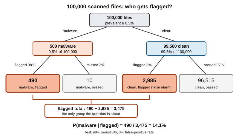
Bayes' theorem through a 100,000-file table: a 98%-sensitive malware test with 3% false alarms and 0.5% prevalence gives 14.1% real flags; a 1,000,000-draw simulation gave 14.4%.
Bayes' theorem converts P(evidence | hypothesis) into P(hypothesis | evidence): P(A|B) = P(B|A) x P(A) / P(B), weighting by the prior and dividing by the total probability of the evidence. The detail interviewers expect is base rates: a detector with 98% sensitivity, 3% false positives and 0.5% prevalence gives only 14.1% real hits among flags.
Bayes' theorem turns P(evidence | hypothesis) into P(hypothesis | evidence) by weighting with the prior and dividing by the total probability of the evidence. For a detector with 98% sensitivity, a 3% false-positive rate and 0.5% prevalence, only 14.1% of flagged files are real malware, and a 1,000,000-draw simulation gave 14.4%, close to the exact 14.1%.
- Bayes' theorem states P(A|B) = P(B|A) x P(A) / P(B), where P(A) is the prior, P(B|A) the likelihood, P(B) the evidence and P(A|B) the posterior.
- For a malware detector with 98% sensitivity, a 3% false-positive rate and 0.5% prevalence, only 490 of 3,475 flagged files per 100,000 are real malware, or 14.1%.
- The law of total probability gives P(B) = P(B|A)P(A) + P(B|not A)P(not A); forgetting the second term, the false alarms, is the most common slip.
- For the same 98%-sensitive test, the share of flags that are real rose from 3.17% at 0.1% prevalence to 97.03% at 50%, while accuracy stayed between 0.970 and 0.975.
- Independent events satisfy P(A|B) = P(A), while mutually exclusive events with nonzero probability are dependent, because one occurring rules out the other.
- If a family has two children and at least one is a girl, the probability both are girls is 1/3; if the older child is a girl, it is 1/2.
01The question and the wrong instinct
A security team scans files with a malware detector. It catches 98% of real malware. It wrongly flags 3% of clean files. About 0.5% of all files are malware. One file gets flagged. What is the chance it is really malware?
Most people say 98%, or something close. That answer is the probability of a flag given malware, and the question asks for the reverse: malware given a flag. The correct figure here is 14.1%. Six in seven flags are false alarms.
This is called base-rate neglect, and it is common even among people who have studied statistics. Mike and Hazzan, at the Technion, tested it in an introductory machine learning course. In the first phase of their study (98 students) only 39% answered their detector question correctly, and the single most popular wrong answer, chosen by 32%, was 95%, the detector's stated accuracy. In a second phase with 153 participants, the question asked in probabilities was answered correctly by 50%, and the version phrased as counts of cases by 58%. The gain is modest, but it points the same way. So the formula is not the only obstacle. The obstacle is keeping track of which group you are dividing by.
02Conditional probability from counts
P(A|B), read "probability of A given B", is a ratio of counts. Take only the cases where B is true. Among them, count those where A is also true. Divide.
P(A|B) = (cases with A and B) / (cases with B)
In symbols that is P(A and B) / P(B), valid when P(B) is above zero. The denominator is the whole point. P(flag | malware) divides by the number of malware files. P(malware | flag) divides by the number of flagged files. Different crowds, different answers, even though the numerator (malware files that were flagged) is the same in both.
Two phrases that interviewers like to mix up deserve their own lines. Independent events: knowing B tells you nothing about A, so P(A|B) = P(A). Mutually exclusive events: A and B cannot both happen. If both have nonzero probability, exclusive events are dependent, because learning that B happened tells you for certain that A did not. A single die roll shows it: "rolls a 2" and "rolls a 5" are exclusive, and given the first, the chance of the second drops from 1/6 to zero.
A quick check on the direction of conditioning is to read the sentence aloud and ask what the denominator crowd is. If you cannot name it, you have not defined the question yet.
03Bayes' theorem as updating proportions
Start from the definition used twice. P(A and B) can be written as P(A|B)P(B) or as P(B|A)P(A). Set them equal and divide:
P(A|B) = P(B|A) x P(A) / P(B)
Four named parts. The prior P(A) is what you believed before the evidence: 0.5% of files are malware. The likelihood P(B|A) is how probable the evidence is if the hypothesis is true: 98% of malware gets flagged. The evidence P(B) is the overall probability of seeing it, flagged or not. The posterior P(A|B) is the updated belief.
For the detector: 0.005 x 0.98 = 0.0049 is the share of all files that are flagged malware. 0.995 x 0.03 = 0.02985 is the share that are flagged clean files. Add them, 0.03475, and the posterior is 0.0049 / 0.03475 = 0.141.
The posterior depends on both the test and the prior. A strong test raises it, but a tiny prior means false alarms from the large clean group still dominate the true hits from the small sick group.
If an interviewer asks you to name the prior, point at the 0.5% and say it is the share of malware before any scan runs. Then say the denominator holds both groups, clean files as well as malware.
04The four-step table routine
Under time pressure, skip the algebra. Use these four steps.
- Pick a round population big enough to avoid fractions. For 0.5% prevalence, 100,000 files.
- Split by prior. 0.5% of 100,000 is 500 malware, leaving 99,500 clean.
- Apply the test to each group. 98% of 500 is 490 flagged, 10 missed. 3% of 99,500 is 2,985 flagged, 96,515 passed.
- Keep only the group the question is about, the flagged files: 490 + 2,985 = 3,475. The answer is the real ones divided by that total: 490 / 3,475 = 14.1%.
The diagram shows the same tree. Notice that the two highlighted boxes are the only ones that matter after the flag; the other two boxes drop out of the problem the moment you are told the file was flagged.
A simulation of 1,000,000 files (NumPy, seed 42) checks the arithmetic. The simulate function below is reused in the next section.
import numpy as np

def exact(prev, sens, fpr):
    return prev * sens / (prev * sens + (1 - prev) * fpr)

def simulate(prev, sens, fpr, n=1_000_000, seed=42):
    rng = np.random.default_rng(seed)
    sick = rng.random(n) < prev
    u = rng.random(n)
    flagged = np.where(sick, u < sens, u < fpr)
    hits = (sick & flagged).sum()
    precision = hits / flagged.sum()
    accuracy = (sick == flagged).mean()
    return precision, accuracy, sick.sum(), flagged.sum(), hits

p, acc, sick, flagged, hits = simulate(0.005, 0.98, 0.03)
print(f"malware {sick:,}  flagged {flagged:,}  real among flagged {hits:,}")
print(f"simulated {p:.4f}  exact {exact(0.005, .98, .03):.4f}")
Output:
malware 5,110  flagged 34,778  real among flagged 5,008
simulated 0.1440  exact 0.1410
Of the 5,110 malware files, 5,008 were among the 34,778 flagged: 0.1440 against the exact 0.1410. The gap is ordinary sampling noise; with only 5,110 sick cases, a swing of a few tenths of a percentage point is expected.
05Total probability and the prevalence sweep
The law of total probability says P(B) = P(B|A)P(A) + P(B|not A)P(not A). In the table routine, that sum is the flagged total of 3,475. Forgetting the second term, the false alarms from the healthy group, is the most common slip. Dividing by P(B|A)P(A) alone gives a posterior of 100%.
The same test, 98% sensitivity and a 3% false-positive rate, behaves very differently as prevalence changes. This loop reuses exact and simulate from the previous section. Each call reseeds the generator with 42, so every row can be reproduced alone, and it prints the exact Bayes value, the simulated precision and the overall accuracy (share of all files classified correctly).
print("prev    exact   simulated  accuracy")
for prev in (0.001, 0.01, 0.1, 0.5):
    p, acc, *_ = simulate(prev, 0.98, 0.03)
    print(f"{prev:<7} {exact(prev, .98, .03):.4f}  {p:.4f}     {acc:.4f}")
Its output:
prev    exact   simulated  accuracy
0.001   0.0317  0.0317     0.9701
0.01    0.2481  0.2494     0.9702
0.1     0.7840  0.7834     0.9710
0.5     0.9703  0.9701     0.9748
Accuracy stayed between 0.970 and 0.975 across all four rows, while the chance that a flag is real went from about 3% to about 97%. A single accuracy figure tells you almost nothing about a rare-event detector, so ask for sensitivity, specificity and prevalence separately.
06Repeated tests and the independence catch
If you rerun the detector and the same file is flagged again, you can treat 14.1% as the new prior. Feeding it back through the formula gives 84.3% after a second flag and 99.4% after a third. This is why a cheap first screen followed by a confirmation step works so well in practice.
There is a condition. The multiplication only works if the two tests are conditionally independent given the file's real status. If the second scan runs the same signature database over the same bytes, a clean file that tripped the first scan will trip the second one too, and the second flag adds almost no information. Two scans from engines that look at different features, or two lab tests that use different chemistry, are the case where the update is legitimate.
A related trap is the conditional puzzle: a family has two children and at least one is a girl; what is the probability both are girls? Counting the equally likely pairs gives 1/3, not 1/2. A simulation shows the two readings differ:
import numpy as np
rng = np.random.default_rng(7)
n = 1_000_000
older = rng.integers(0, 2, n)    # 1 = girl
younger = rng.integers(0, 2, n)
both = (older == 1) & (younger == 1)
at_least_one = (older == 1) | (younger == 1)
print(f"at least one girl: {both[at_least_one].mean():.4f}")
print(f"older is a girl:   {both[older == 1].mean():.4f}")
at least one girl: 0.3333
older is a girl: 0.4996The two sentences select different crowds, which is the same lesson as the detector in a smaller package.
07Link to machine learning: precision and Naive Bayes
In classification terms, sensitivity is recall: P(flag | positive). The false-positive rate is 1 minus specificity. And precision, the share of flagged items that are truly positive, is exactly the Bayesian posterior we computed: 14.1% for our detector. The Logistic Regression and Classification Metrics topic covers precision and recall in full. This is why a classifier with 98% recall can still have poor precision on imbalanced data, and why interviewers ask "what happens to precision if prevalence drops by ten?" Hold recall and false-positive rate fixed, and precision falls with prevalence, as the sweep table showed.
Naive Bayes is Bayes' theorem applied to text. For a message, the classifier scores P(spam | words) as proportional to P(spam) times the product of P(word | spam). The "naive" assumption is that words are independent given the class. That is false for real language, but it makes the likelihood easy to estimate, and the ranking of classes often survives the error.
Here is a toy, not a real spam filter: three hand-written spam messages, three ham messages, a 12-word vocabulary, equal priors, Laplace smoothing (add 1 to every count).
import math
spam = ["win cash now", "win a prize now", "cheap cash prize"]
ham  = ["meeting at noon", "lunch at noon now", "project meeting notes"]

def counts(docs):
    c = {}
    for d in docs:
        for w in d.split():
            c[w] = c.get(w, 0) + 1
    return c

cs, ch = counts(spam), counts(ham)
V = set(cs) | set(ch)

def p_spam(msg, k=1):
    ls = lh = math.log(0.5)
    ts, th = sum(cs.values()), sum(ch.values())
    for w in msg.split():
        ls += math.log((cs.get(w, 0) + k) / (ts + k * len(V)))
        lh += math.log((ch.get(w, 0) + k) / (th + k * len(V)))
    return 1 / (1 + math.exp(lh - ls))

print("vocabulary size:", len(V))
for m in ("win cash prize", "meeting now", "win meeting noon", "cheap meeting"):
    print(f"{m!r}: {p_spam(m):.3f}")
try:
    p_spam("cheap meeting", k=0)
except ValueError as e:
    print("k=0 on 'cheap meeting':", e)
Output:
vocabulary size: 12
'win cash prize': 0.964
'meeting now': 0.333
'win meeting noon': 0.250
'cheap meeting': 0.400
k=0 on 'cheap meeting': math domain error
With k=0 the word "cheap" never appears in ham, so its ham probability is zero and log(0) is undefined. With smoothing the same message scores 0.4. That is the zero-probability problem, and smoothing is the standard fix. Logs are used because multiplying many small probabilities underflows.
One more link: a p-value answers "how surprising is this data if the null hypothesis is true", which is P(data | hypothesis), not the posterior P(hypothesis | data). The same direction mix-up from the first section applies; the A/B Testing and Statistical Significance topic shows where it bites.
08Common interview questions
Q: What is the difference between P(A|B) and P(B|A)?
A: They divide by different groups. P(A|B) is the share of B cases that also have A; P(B|A) is the share of A cases that also have B. Bayes' theorem converts one into the other using the priors: P(A|B) = P(B|A) P(A) / P(B). Confusing them is the prosecutor's fallacy.
Q: A test has 98% sensitivity and a 3% false-positive rate, and 0.5% of items are positive. A test result comes back positive. What is the probability it is a true positive?
A: Take 100,000 items: 500 positive, 490 caught; 99,500 negative, 2,985 falsely flagged. The answer is 490 / (490 + 2,985) = 14.1%.
Q: Are independent events the same as mutually exclusive events?
A: No. Independent means P(A|B) = P(A). Mutually exclusive means P(A and B) = 0. If both events have nonzero probability, exclusive events are dependent, since one occurring rules out the other.
Q: A family has two children and at least one is a girl. What is the chance both are girls?
A: 1/3. The equally likely outcomes consistent with the information are girl-girl, girl-boy and boy-girl. If you are told a specific child, such as the older one, is a girl, the answer becomes 1/2.
Q: Why does precision depend on class prevalence but recall does not?
A: Recall divides by the actual positives, so prevalence cancels out. Precision divides by all flagged items, which includes false alarms drawn from the negative class. A larger negative class produces more false positives at a fixed false-positive rate, so precision falls.