Transformers and Self-Attention
Self-attention scores every token pair, softmaxes the scores and mixes value vectors. In a simulation, q.k variance tracked d_k (1033 at d_k=1024), which is why scores are scaled by sqrt(d_k).
Self-attention lets every token weigh every other token in one step: it takes dot products of queries and keys, scales them by sqrt(d_k), applies softmax to get weights, and outputs a weighted sum of value vectors. Interviewers expect the reason for the scaling: without it, large scores saturate softmax toward one-hot, where gradients are tiny.
Self-attention lets every token look at every other token in a single step: it scores pairs with dot products, softmaxes the scores into weights, and averages value vectors. This page works one head by hand on three tokens, then measures why scores are scaled by sqrt(d_k), how position gets in, and how cost grows with sequence length.
- Scaled dot-product attention is defined in the 2017 paper Attention Is All You Need as softmax(Q K^T / sqrt(d_k)) V.
- Per layer, self-attention costs O(n^2 d) with O(1) sequential operations and path length, while a recurrent layer costs O(n d^2) with O(n) of each.
- For independent unit-variance components, a query-key dot product has variance d_k; a simulation measured 1033 at d_k = 1024.
- The original Transformer base model uses d_model = 512 with 8 attention heads of d_k = d_v = 64, and stacks 6 layers in both encoder and decoder.
- Self-attention alone is permutation-equivariant, so Transformers add positional encodings, sinusoidal in the original paper, to tell token order apart.
- A causal mask sets attention scores for future positions to minus infinity before softmax, so decoder weights become lower-triangular.
01What the Transformer replaced
A recurrent network reads a sentence one token at a time and carries a hidden state forward. Two things follow. Training cannot be parallelised along the sequence, because step 5 needs the state from step 4. And when token 1 matters for token 50, the signal has to survive 49 updates.
The 2017 paper "Attention Is All You Need" (Vaswani et al.) proposed the Transformer, a model built only on attention, with no recurrence and no convolution. Its Table 1 compares layer types. Self-attention costs O(n^2 d) per layer, with O(1) sequential operations and a maximum path length of O(1) between any two positions. A recurrent layer costs O(n d^2), needs O(n) sequential operations and has a path length of O(n). Here n is the sequence length and d the vector width.
In short: you pay quadratically in sequence length, and in exchange you get parallel training and short paths. When n is smaller than d, which was the usual case for sentence-level translation, attention is even the cheaper layer per step. The paper reported 27.3 BLEU for the base model on WMT14 English-to-German and 28.4 for the big one.
This is the first Advanced topic in the AI & ML path, so it assumes you know how a network is trained. If gradients and backpropagation feel shaky, read the gradient-descent-and-backpropagation topic first.
02One attention head, computed by hand
Take three tokens with 2-dimensional vectors: A = [1,0], B = [0,1], C = [1,1]. To keep the arithmetic visible, let the three projection matrices be the identity, so Q = K = V = X. (Real models learn them; this is only for hand-checking.)
import numpy as np

def softmax(x):
    e = np.exp(x - x.max(-1, keepdims=True))
    return e / e.sum(-1, keepdims=True)

X = np.array([[1, 0], [0, 1], [1, 1]], float)   # tokens A, B, C
Q = K = V = X                                    # identity projections
scores = Q @ K.T
weights = softmax(scores / np.sqrt(K.shape[1]))
print(weights.round(3))
print((weights @ V).round(3))
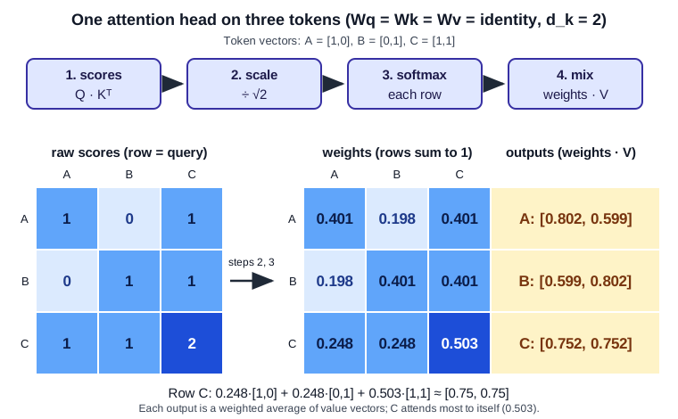
Step one is the score matrix Q K^T. The score of row i, column j is the dot product of token i's query with token j's key. Running this in NumPy gives
A: [1, 0, 1]
B: [0, 1, 1]
C: [1, 1, 2]
Step two divides by sqrt(d_k) = sqrt(2), giving 0.707, 0 and 1.414 as the distinct values. Step three applies softmax to each row. Row C becomes [0.248, 0.248, 0.503], and every row sums to 1. Step four multiplies the weight matrix by V. Output C is 0.248 x [1,0] + 0.248 x [0,1] + 0.503 x [1,1], which is [0.752, 0.752]. Output A comes out as [0.802, 0.599] and B as [0.599, 0.802].
Token C, which contains both A and B, spread its attention across all three and gave itself the largest share. Nothing here was learned. The mechanism is just similarity, normalised, then used to mix vectors. The diagram shows the four steps with these exact numbers.
03Queries, keys and values
A Python dict returns the value whose key matches your query exactly. Attention does the fuzzy version. Each token produces three vectors from its input x using three learned matrices: a query q = x Wq, a key k = x Wk and a value v = x Wv. The query says what this token is looking for. The key says what this token offers to others. The value is what actually gets passed along if it is picked.
Separating the roles gives the model freedom. A token can be easy to find (a distinctive key) while carrying a different payload (its value). In the hand example above all three were identical, which is why it is a poor model of language but a good one of arithmetic.
In matrix form, for a whole sequence at once, the paper writes Attention(Q, K, V) = softmax(Q K^T / sqrt(d_k)) V. A random 4-token case (rng = np.random.default_rng(1), X of shape (4, 8) from standard normals, and Wq, Wk, Wv of shape (8, 4) drawn from the same generator in that order) shows the shapes. Q, K and V each have shape (4, 4). The code is rng = np.random.default_rng(1); X = rng.standard_normal((4, 8)); Wq, Wk, Wv = (rng.standard_normal((8, 4)) for _ in range(3)); Q, K, V = X @ Wq, X @ Wk, X @ Wv. The raw score matrix ran from -10.86 to 20.54, the softmaxed weights were 4 x 4 with each row summing to 1, and the output was again 4 x 4, one new vector per token. With random projections the weights are lopsided: the last two rows put essentially all their weight on the last token. Your numbers will differ with another seed. The score matrix is n by n, which is where the quadratic cost comes from.
04Why divide by the square root of d_k
The paper gives the argument. If the components of q and k are independent with mean 0 and variance 1, the dot product has mean 0 and variance d_k. Wide heads therefore produce large scores, and softmax of large numbers is nearly one-hot, a region where gradients are extremely small. (The gradient-descent-and-backpropagation topic explains why tiny gradients stall training.)
I checked this with a simulation, not a trained model. For each d_k I drew 20,000 pairs of random unit-variance vectors and measured the variance of q.k. Then I took 2,000 queries, each against 10 random keys, and measured the average largest softmax weight, with and without the 1/sqrt(d_k) factor. This is the code, with the seed:
rng = np.random.default_rng(0)
for dk in (4, 16, 64, 256, 1024):
    q = rng.standard_normal((20000, dk)); k = rng.standard_normal((20000, dk))
    var = (q * k).sum(1).var()                      # variance of q.k
    qq = rng.standard_normal((2000, dk))            # 2000 queries ...
    kk = rng.standard_normal((2000, 10, dk))        # ... each against 10 keys
    sc = np.einsum('nd,nkd->nk', qq, kk)
    print(dk, round(var, 2), softmax(sc).max(1).mean().round(2),
          softmax(sc / np.sqrt(dk)).max(1).mean().round(2))
Output, one row per d_k (variance, max weight unscaled, max weight scaled):
d_k = 4: 4.0, 0.50, 0.31
d_k = 16: 16.25, 0.72, 0.31
d_k = 64: 63.38, 0.86, 0.32
d_k = 256: 258.31, 0.93, 0.32
d_k = 1024: 1033.0, 0.97, 0.32
The measured variance tracks d_k closely, with sampling noise of a few percent. Without scaling, the biggest weight climbs toward 1.0, so one key takes nearly everything. With scaling it stays near 0.32 whatever the width. The factor exists to keep the score spread constant as the head widens, so softmax can still learn. This simulation shows the forward behaviour only; it does not measure gradients.
05Multi-head attention
One softmax per token produces one distribution, so a single head must squeeze every kind of relationship into one set of weights. Multi-head attention runs h heads side by side. Each has its own Wq, Wk and Wv that project the input to a smaller size, each computes attention independently, and the results are concatenated and passed through a final matrix W^O.
The paper's base model uses d_model = 512 and h = 8 heads with d_k = d_v = 64, so the heads together are as wide as the model and the compute is close to a single full-width head. Counting parameters on a toy version confirms the budget: with d_model = 8, one head with full-width Wq, Wk, Wv and Wo has 4 x 8 x 8 = 256 weights. Two heads of width 4, with their three projections (8 x 4 each) plus the 8 x 8 output matrix, also total 256.
Because each head has its own Wq, Wk and Wv, each one scores token pairs in its own subspace and produces its own weight matrix, so two heads can attend to different tokens for the same query. In practice no loop over heads is needed. You compute one full-width Q, K and V, reshape the d_model axis into h slices of d_model/h, and run a single batched matmul over the head axis. In my NumPy check, d_model = 8 and h = 2 turned (4, 8) projections into score tensors of shape (2, 4, 4), and the concatenated output was (4, 8) again. This page does not inspect trained heads, so it makes no claim about which patterns they find, and it does not test whether attention weights explain a model's decision.
06Position: attention cannot see order
Shuffle the tokens, run attention, and you get the same outputs shuffled the same way. Self-attention is permutation-equivariant. The permutation test (seed 2, random 8 x 8 projections): with 4 tokens, permuting the input rows and permuting the output rows gave identical results (allclose returned True). Left alone, the model could not tell "dog bites man" from "man bites dog".
The fix is to inject position. The paper adds a fixed vector to each embedding: PE(pos, 2i) = sin(pos / 10000^(2i/d_model)) and PE(pos, 2i+1) = cos of the same angle. Early dimensions oscillate fast and later ones slowly, so each position gets a distinct pattern. For d_model = 8, the code prints position 0 as [0, 1, 0, 1, 0, 1, 0, 1] and position 1 as [0.841, 0.540, 0.100, 0.995, 0.010, 1.000, 0.001, 1.000].
After adding these, the same test fails: the shuffled input no longer gives shuffled outputs (allclose returned False), because the model now sees where each token sat. The decoder also needs to be stopped from looking ahead, which is the causal mask in the next section.
07The full block, masking and cost
The paper stacks N = 6 identical layers in the encoder and in the decoder. Each layer wraps each of its two sublayers, attention and then a position-wise feed-forward network (d_ff = 2048 in the base model), as LayerNorm(x + Sublayer(x)): a residual connection followed by layer normalisation (Vaswani et al., 2017). The encoder reads the whole input at once. The decoder generates output one token at a time, so during training it must be stopped from peeking at later positions.
The causal mask does that. Before softmax, scores for future positions are set to minus infinity, so their weights become exactly 0:
s = Q @ K.T / np.sqrt(K.shape[1])
s = np.where(np.triu(np.ones(s.shape, bool), k=1), -np.inf, s)   # block j > i
weights = softmax(s)
On the random 4-token example from earlier (same seed), the weights came out lower-triangular: row 0 was [1, 0, 0, 0], row 1 was [0.24, 0.76, 0, 0], row 2 was [0.94, 0.001, 0.06, 0], and row 3 was about [0, 0, 0.001, 0.999] (rounded). Which entries are nonzero is fixed by the mask; the sizes depend on the seed.
Encoder and decoder differ in what they attend to. Encoder self-attention is unmasked. Decoder self-attention is masked. A standard encoder-decoder model adds a third sublayer in the decoder, cross-attention, where the queries come from the decoder and the keys and values come from the encoder's output, which is how a translation can look back at the source sentence. GPT-style decoder-only models drop the encoder and cross-attention entirely and use only masked self-attention over one sequence.
Now the cost. Attention builds an n x n score matrix, so time and memory grow with n squared, not with d squared. Timing a single head with d = 64 on a 2-core CPU (OMP_NUM_THREADS=1, NumPy 2.5.3), with 3 warm-up calls and the median of 30 runs of the function above:
n = 128: 0.28 ms
n = 256: 1.09 ms (3.9x)
n = 512: 4.38 ms (4.0x)
n = 1024: 33.47 ms (7.6x)
n = 2048: 154.65 ms (4.6x)
n = 4096: 1238.03 ms (8.0x)
The n^2 growth is visible, with the first two doublings close to the expected 4x. The later ones are noisier and larger than 4x. The fastest single runs at 1024 and 4096 were 29.25 ms and 665.26 ms, so the medians include machine noise. Another run on the same machine gave 111.6 ms at n = 2048 and 465.5 ms at n = 4096, so absolute times are unreliable, and possible causes such as cache effects were not tested. Treat this as one noisy machine, not a benchmark.
08Common interview questions
Q: What do queries, keys and values do?
A: A query is what a token looks for, a key is what it offers for matching, and a value is the content passed on. Softmax of query-key dot products gives weights, and the output is the weighted sum of values.
Q: Why divide by sqrt(d_k)?
A: For independent, zero-mean, unit-variance components the dot product has variance d_k. Large scores saturate softmax towards one-hot, where gradients are tiny. Dividing by sqrt(d_k) restores variance near 1.
Q: Why multi-head attention instead of one big head?
A: Each head projects into its own subspace and produces its own weights, so the model can capture several relationships at once. With h heads of size d_model/h the cost stays close to one full-width head.
Q: How does a Transformer know word order?
A: Self-attention alone is permutation-equivariant, so position vectors, sinusoidal in the original paper, are added to the embeddings before the first layer.
Q: Compare self-attention and recurrence.
A: Per layer, attention is O(n^2 d) with O(1) sequential steps and O(1) path length. Recurrence is O(n d^2) with O(n) sequential steps and O(n) path length. Attention parallelises and links distant tokens directly but is quadratic in n.
Q: What is the difference between self-attention and cross-attention?
A: In self-attention, queries, keys and values all come from the same sequence. In cross-attention, queries come from the decoder and keys and values come from the encoder output, so the decoder can read the source. Decoder-only models such as GPT-style ones have no cross-attention.